Empirical Copula Estimation
Introduction
In this post, I’d like to discuss empirical copula density estimation from data. We will introduce the concept of copulas, the copula density estimation problem, and how to solve it. We will also detail an implementation of the proposed solution in Matlab. All code used in this post is taken from the Matlab copula toolbox that I developed as part of my PhD research.
Sadly, I don’t have an opportunity to maintain this toolbox anymore, but I highly recommend using R for any copula based computing needs you might have. The amount of available packages far surpasses what is available in Matlab.
Copula Background
Copulas are functions which capture the dependence structure of joint distribution functions. They can also be seen as multivariate probability distribution functions with marginal distributions that are uniform. These equivalent descriptions of copulas can be expressed mathematically through Sklar’s theorem:
\[C(F_{X_1}(x_1), \dots, F_{X_d}(x_d)) = F_{X_1, \dots, X_d}(x_1, \dots, x_d) \ \ \ \ \ \ \ \ \ \ \ [1]\]If we define \(u_i = F_{X_i}(x_i)\), then Sklar’s theorem can be restated as
\[C(u_1, \dots, u_d) = F_{X_1, \dots, X_d}(F^{-1}(u_1), \dots, F^{-1}(u_d))\ \ \ \ \ \ \ \ \ \ \ [2]\]Equation [1] and [2] are equivalent and show that any joint distribution \(F_{X_1, \dots, X_d}(x_1, \dots, x_d)\) can be expressed with the joint distribution’s copula function \(C\) and the marginal distributions \(F_{X_i}(x_i)\). The perceptive reader may notice that there was an implication of the uniqueness between a joint distribution \(F_{X_1, \dots, X_d}(x_1, \dots, x_d)\) and its copula \(C\) in the previous statement. To be precise, Sklar’s theorem guarantees that if the marginal distributions \(F_{X_i}(x_i)\) for all \(i\) are continuous random variables, then \(C\) is unique. In this post, we will assume that \(X_i\) for all \(i\) are continuous random variables.
Problem Description
Although Sklar’s theorem, shown above in Equations [1] and [2], guarantees a unique copula \(C\) for any joint distribution \(F_{X_1, \dots, X_d}(x_1, \dots, x_d)\) (provided the marginal distributions \(F_{X_i}(x_i)\) are continuous random variables), it does not describe how to find this unique copula. In fact, copula model selection (i.e. which copula to use) is a significant area of research. In general, there are two solutions to copula model selection:
- Choose a copula among existing copula families such as Gaussian, t, or Archimedean copulas which fit the data well, using some metric to decide between the copula families.
- Calculating an empirical copula.
The advantages and disadvantages of each approach is out of the scope of this post. Rather, we will focus on the second approach, which is calculating an empirical copula, and more specifically, an empirical copula density. This can be considered as a nonparametric approach.
The empirical copula can be thought of as an estimate of the underlying dependency structure of the data, unconstrained by any a-priori models of how the data interacts with each other. In this light, it is similar to a kernel density estimate because the copula function (and copula density function) can be thought of as a distribution function (and density function) itself.
The Empirical Copula Density Estimation Problem
Before describing the copula density estimation problem, it is useful to summarize the problem statement mathematically. Suppose we have a multivariate dataset \(\mathbf{X} \in \mathbb{R}^d\) in an \(n \times d\) matrix, where each column \(X_i\) is a “feature,” and there are \(d\) features and \(n\) sample points per feature. We would like to estimate the copula density \(c(\mathbf{u}) = \frac{\partial C(\mathbf{u})}{\partial \mathbf{u}}\) which captures the dependency between the columns in the dataset \(\mathbf{X}\). How would we go about approaching this problem?
The Solution
There are many solutions to the problem posed above. We discuss two approaches here, and outline why the naive approach may not be a good idea for estimating copula densities.
The Naive Approach
The naive approach entails calculating the empirical copula function and then performing differentiation:
\[\hat{c}(\mathbf{u}) =\frac{\partial \hat{C}(\mathbf{u})}{d \mathbf{u} } = \frac{1}{n} \frac{\partial}{d \mathbf{u}} \sum_{i=1}^n \mathbf{I}(\tilde{U}_1^i \leq u_1, \dots,\tilde{U}_d^i \leq u_d)\ \ \ \ \ \ \ \ \ \ \ [3]\] \[(\tilde{U}_1^i \leq u_1, \dots,\tilde{U}_d^i \leq u_d) = (F_1^n(X_1^i),\dots,F_d^n(X_d^i))\ \ \ \ \ \ \ \ \ \ \ \ \ [4]\]where Equation [4] is an expression for the pseudo copula observations. While this is tempting, discontinuities in data can lead to differentiability issues. Additionally, even if discontinuities are not present in the data, the copula density derived by numerical differentiation of the empirical copula function will be spiky. The spiky nature of the numerical derivative is simply a consequence of the algorithm that is used for differentiation. We will see an example of the effect of numerical differentiation on an empirical copula below.
Of course, more sophisticated techniques such as second order approximations can be implemented and they may yield acceptable solutions. However, there exists a more natural approach to estimating the copula density from data directly.
Direct Density Estimation
An alternative to the approach described above is to estimate the density directly from data using kernel methods. For copula density estimation, it is preferred to use the Beta kernel, because both the Beta kernel and the copula have a bounded support on the interval \([0,1]\), which eliminates boundary bias. Additionally, the Beta kernel can be viewed as an adaptive kernel density estimation approach, because it changes shape with respect to the input, even if the kernel density estimation bandwidth, \(h\), remains the same. For more details, please see References 1 and 2 below.
The formula then for multivariate copula density estimation is:
\[\hat{c}_\beta(\mathbf{u}) = \frac{1}{N} \sum_{n=1}^N \prod_{d=1}^D \beta(F_d(x_d(n)), \frac{u}{h} + 1, \frac{1-u}{h} + 1)\ \ \ \ \ \ \ \ \ \ \ [5]\]where \(h\) is the kernel bandwidth parameter, \(\beta\) is the probability density function of the Beta distribution, and \(F_d(x_d(n))\) is the \(n^{th}\) pseudo observation in dimension \(d\). Equation [5] is nothing more than a multivariate kernel density estimate of the data, using beta kernels. However, it has the advantages stated above:
- Eliminates boundary bias,
- Adaptive approach to density estimation
- It is shown in the references below that the variance of the estimator decreases with increased sample size.
Implementation
Any copula operations depend upon \(u_i\) rather than \(x_i\). The \(u_i\)’s are termed pseudo observations, and there are two ways of estimating them. We discuss the pros and cons of different ways to estimate the pseudo observations before diving into the details of estimating the copula function and the copula density directly.
Generating Pseudo Observations
There are atleast two ways to generate pseudo observations:
\(U_i = \frac{R_i}{n+1}\) \(U_i = F_{X_i}(x_i[m])\)
The Matlab function pobs has the ability to generate pseudo observations using both methods described above. Briefly, the rank based method (option 1 above) can be implemented as:
U = tiedrank(X)/(M+1); % scale by M+1 to mitigate boundary errors
In the code above, each column is ranked and scaled to achieve a uniform distribution from the observed data. To implement the empirical CDF approach (option 2 above), we do the following
U = zeros(size(X));
for nn=1:N
    domain = linspace(min(X(:,nn)),max(X(:,nn)),numEcdfPts);
    FX = ksdensity(X(:,nn), domain, 'function', 'cdf')';
    empInfoObj = rvEmpiricalInfo(domain, [], FX);
    for mm=1:M
        U(mm,nn) = empInfoObj.queryDistribution(X(mm,nn));
    end
end
It can be seen that the ECDF method requires estimation of each marginal empirical density function, and then querying that distribution for each of the samples. From a computational perspective, the rank approach is faster due to vectorization and modern sorting algorithms being lightning quick!
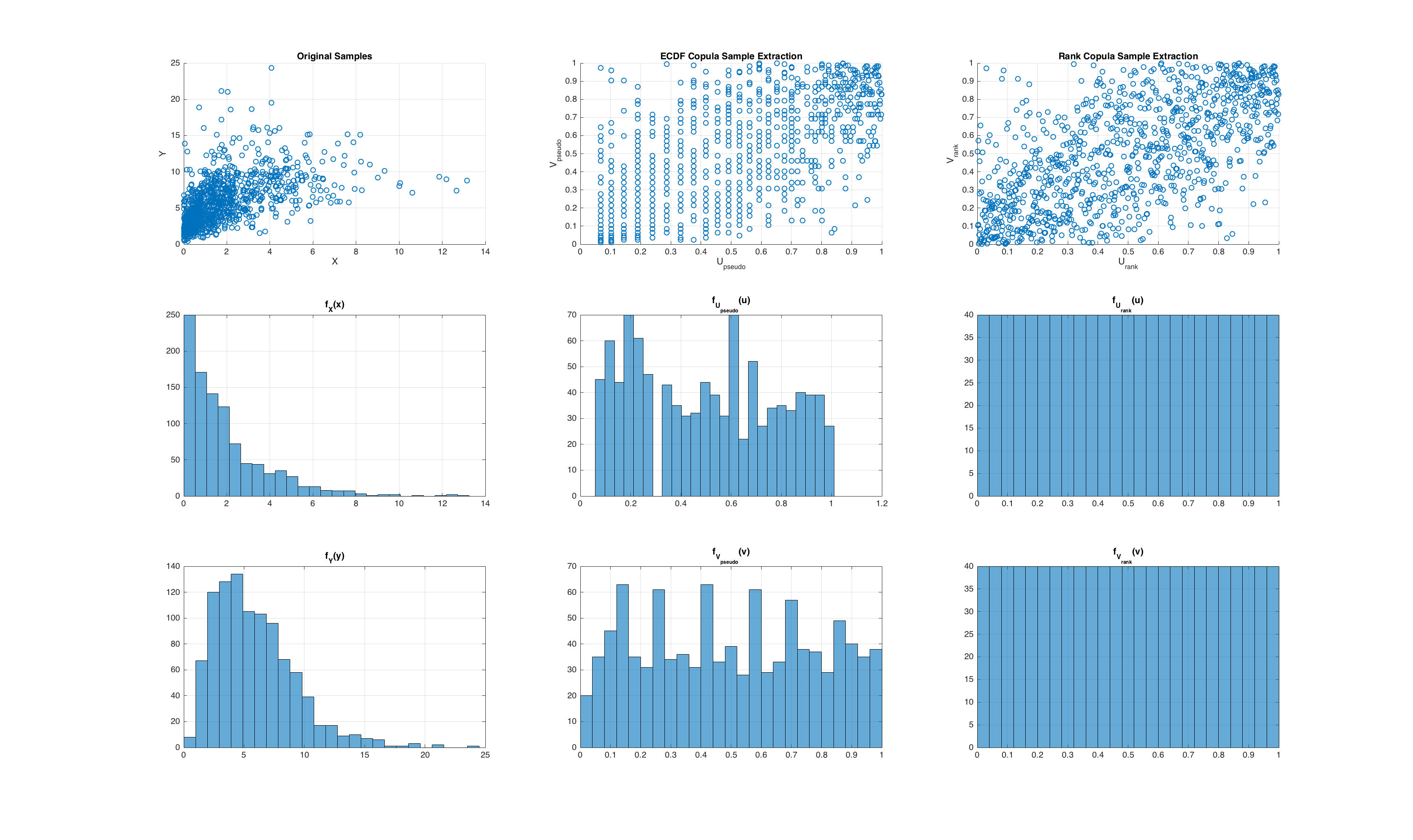
Both are valid approaches to generating pseudo observations, but if we do not know the marginal distributions a-priori (which is usually the case), the rank based approach actually produces a \(U_i\) that is more uniformly distributed than the empirical CDF approach! The rank based approach is able to do this because it evenly distributes the original observations into the unit cube (by virtue of the rank function). To show this in Matlab, we can generate samples from a joint distribution and compute the pseudo observations using both methods, and compare the distributions of the computed pseudo observations. To generate samples from a joint distribution, we can utilize the copularnd function as follows:
M = 1000;
alpha = 5;
u = copularnd('Frank', alpha, M);

mu = 2; a = 3; b = 2;

x = [expinv(u(:,1),mu), gaminv(u(:,2),a,b];
After generating the dependent random variables, we compute the pseudo observations using the pobs function with both the rank algorithm and the ECDF algorithm as follows:
numECDFPts = 100;
U_ecdf = pobs(x, 'ecdf', numECDFPts);
U_rank = pobs(x); % default option for pobs is rank
Finally, we compute an empirical density via a histogram for the two different pseudo observations. The results are shown below.

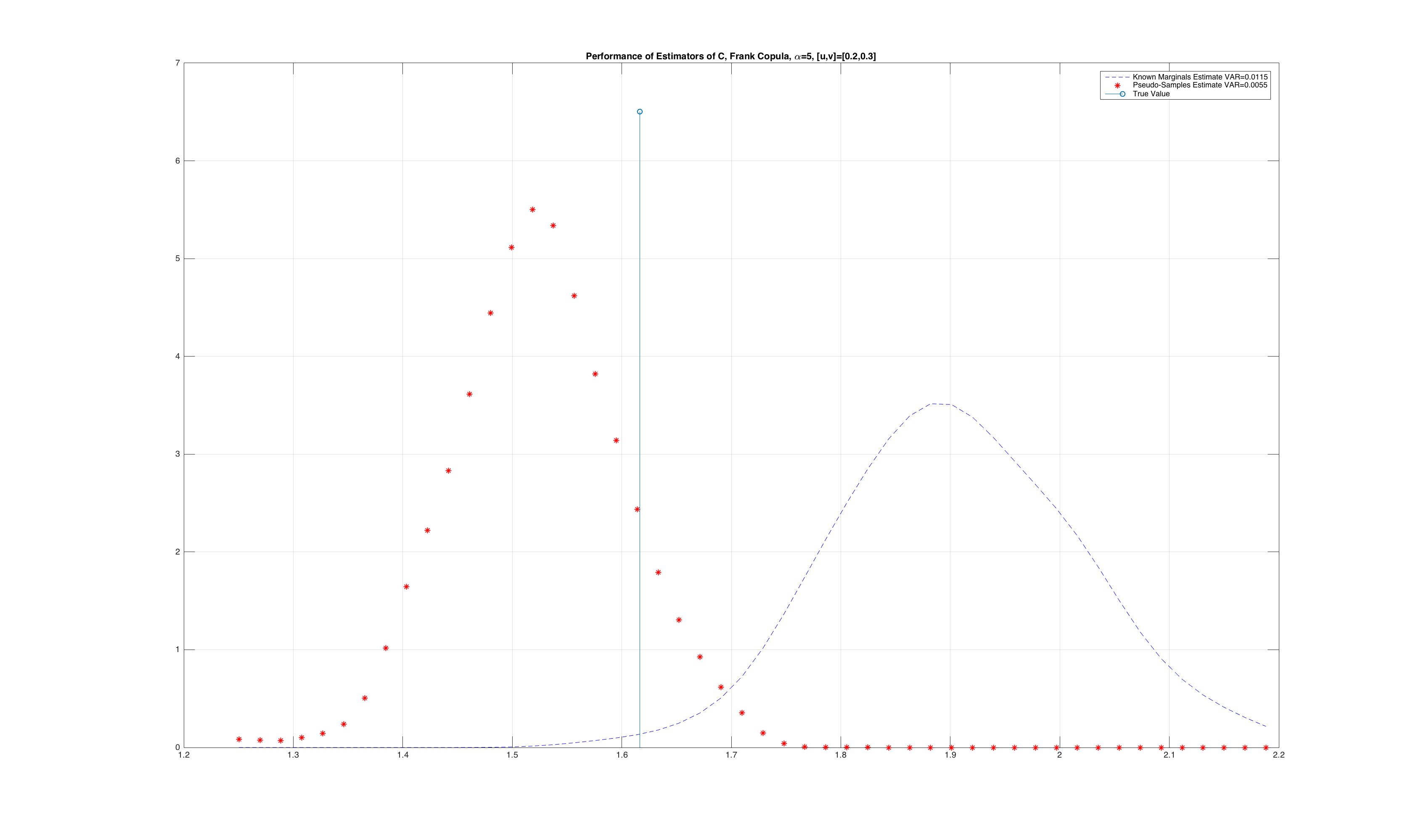
A consequence of “more” uniformity is that the rank based calculation of the pseudo observations actually produces lower variance estimates of an empirical copula estimated with rank based pseudo observations. For intuition on this, please refer to Reference [2]. We empirically show this with a simulation where we generate samples from a joint distribution, and perform a Monte-Carlo simulation where we compare the variance of the estimated value of the original copula density from pseudo observations computed with the ECDF and the rank method. We only demonstrate this for a sample point in the unit cube, but the results apply to the entire space of \(\mathbf{I}^d\). The results are show below:

It is clear from the figure that the variance is lower when using pseudo observations from the rank based estimator. The proof and intuition of using the rank based algorithm for generating pseudo observations is given in Reference [2], and the full simulation to generate the figures above is located here.
Estimation via Empirical Copula Function and Gradients
Having discussed how to generate pseudo observations, let us tackle the problem at hand of estimating the empirical copula density. We first calculate the empirical copula by
\[\hat{C}(\mathbf{u}) = \frac{1}{n} \sum_{i=1}^n \mathbf{I}(\tilde{U}_1^i \leq u_1, \dots,\tilde{U}_d^i \leq u_d)\ \ \ \ \ \ \ \ \ \ \ [6]\]where \(U_i\) are the the pseudo observations. The function empcopulacdf implements Equation [6], and is included in the copula Matlab toolbox. Using this, the pobs function, and gradient, we can easily estimate a copula density from samples as follows:
K = 25;
U = copularnd('Frank', 5, 1000);

C_est = empcopulacdf(U, K, 'deheuvels');
[cc] = gradient(C_est);
[~,c_est_grad] = gradient(cc);
Direct Empirical Copula Density Estimation
To estimate the density directly, we use the empcopulapdf function which implements Equation [5] above. This function has the same call signature as empcopulacdf, and using the same data source as above, we can generate a copula density estimate as follows:
h = 0.05;
c_direct = empcopulapdf(U, h, K, 'betak');
Comparison
Let us now compare these two methods of density estimation by plotting the results, against the true copula density for the Frank copula with a dependency parameter of 5. The figure below shows three plots of the Frank copula. The plot on the left represents the true copula density, the plot in the middle shows the density derived from estimating the empirical copula first and performing directional derivatives, and finally the plot on the right shows the empirical copula density generated from the outlined Beta kernel approach.

The source for generating these diagrams is located in test_empcopulacdf.m.
Conclusion
In this post, we have discussed two different methods for estimating a copula density directly from data. From the limited experiments conducted above, two recommendations can be given:
- Use a rank based approach to generating pseudo observations.
- If the empirical copula density is what is required, estimate it directly from data using the Beta kernel approach outlined above, as opposed to computing the empirical copula function and performing directional derivatives.
In the next post, we’ll discuss the mathematics behind generating random samples from an empirical copula, using the empcopularnd function.