QPSK Burst Receiver Synchronization
Introduction
In this post, I’d like to discuss the signal acquisition algorithms that need to be performed in order to properly receive and demodulate a bursty QPSK signal in a wireless multipath environment.
Background
In the wireless communications world, receiver design is traditionally more complex than transmitter design. This is mainly due to the receiver needing to perform large amounts of pre-processing in order to synchronize itself with respect to time and frequency to the transmitter, as well as account for wireless channel effects such as multipath. Modern wireless communications standards (4G and beyond) have attempted to put more intelligence into the transmitter in order to simplify receiver design, but the fact remains that the receiver still needs to account for these effects.
In this post, we will consider the scenario where we have a burst mode QPSK transmitter and receiver and detail the acquisition algorithms that a receiver would need to perform in order to properly demodulate the signal. Acquisition in a wireless receiver typically refers to time synchronization, frequency synchronization, and accounting for wireless channel effects such as multipath. Let’s discuss each of these effects in detail.
Time Synchronization
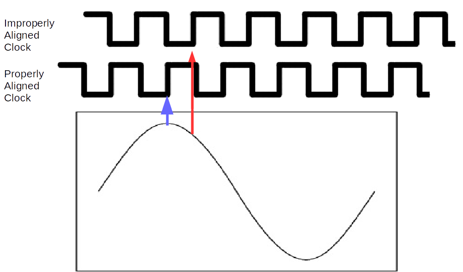
Time synchronization is the process of aligning the receiver sample clock with the transmitter sample clock. It is well known in digital communication theory that sampling at the optimal point gives the receiver the highest probability of making a correct decision on a certain symbol. Intuitively, sampling at the correct moment in time gives the receiver the maximum energy point at which to threshold and make a decision. We illustrate this concept in a simplified example in the diagram below. Suppose that we would like to determine the peak-to-peak voltage of a sinusoid. As seen in the diagram below, if the sample clock is aligned properly, it can be seen that sampling the signal achieves the maximum energy (shown in the blue arrow), while a misaligned clock (shown in the red arrow) will result in reduced energy in the sample.
Frequency Synchronization
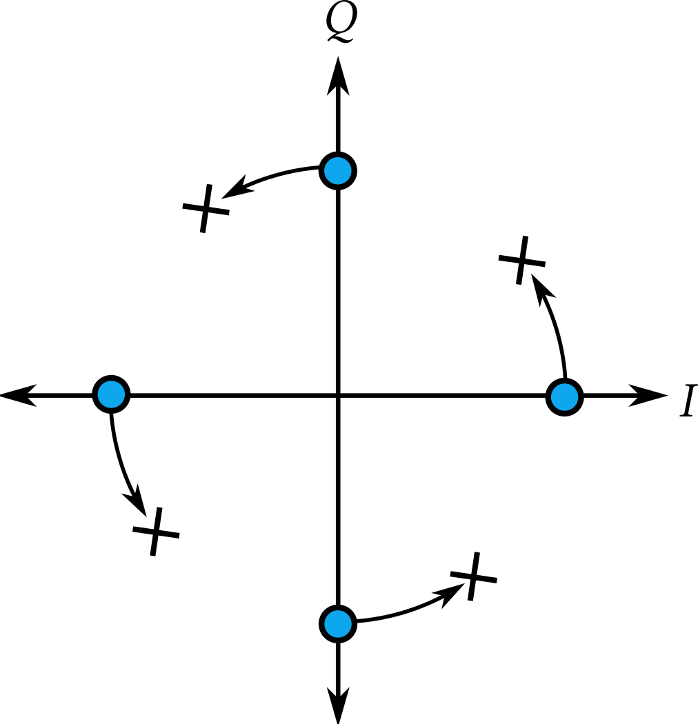
Frequency synchronization refers to ensuring that the receiver is locked and tracking the frequency drift of the transmitter, which can be caused by many real-world effects such as LO drift, Doppler, etc. Again, as is the case with time synchronization, lack of frequency synchronization adversely affects the receiver. A typical symptom of lack of frequency synchronization is a rotating constellation. The effect of a rotating constellation for a receiver is that the receiver will incorrectly map the symbols to bits, because they are perceived to be in different locations on the constellation plane. The figure below shows where actual QPSK points are expected (in the blue dots), and where they would end up with a frequency offset (shown by the X’s). To be clear, a phase mismatch between the transmitter and receiver would result in a static rotation of the constellation, but a center frequency offset would result in a rotating constellation, with the rotation speed proportional to the frequency offset.
An additional complication in a wireless receiver is that the time and frequency corrections need to also be tracked through the entire duration of the transmission being active. In the continuous signaling case (and in some burst cases), this is typically accomplished through the use of a Phase Lock Loop (PLL) and Frequency Lock Loop (FLL) working in conjunction with each other. The PLL/FLL approach works well for continuous signals because once initial synchronization is achieved, the feedback nature of the loops allow the receiver to track the variations. In burst situations however, the transmission toggles between on and off at a certain duty cycle that may or may not be deterministic. If the PLL and FFL’s need more data to synchronize than the initial preamble which is typically present in burst communications, data will be lost. Considering the bursty nature of the signal, we have chosen to use an adaptive filter to perform the bulk of the initial synchronization. It is important to note that we detail just one method of performing acquisition, but that this is not the only approach (or even the best).
At a high level, this approach views acquisition as an FIR filtering problem. The premise is that there is an FIR filter (optimal in the MMSE sense) that can perform time and frequency synchronization, as well as account for wireless channel effects. The question then becomes, what do the FIR filter taps need to be in order to perform acquisition? Another question is, can the taps remain constant, or do they need to change over time? The answers to these questions can be found by reviewing some wireless communication theory.
Theory
A wireless channel can be approximately modeled as a linear system, meaning that mathematically it has impulse response. The impulse response of a wireless channel at a certain time \(T_0\) may look like the diagram below, which shows three multipath components.
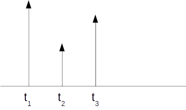
The channel impulse response shown has three multipath components, which means that the receiver will see three copies of the transmitted signal, overlapped on top of each other at different amplitudes. This is the effect of multipath, and needs to be accounted for if a receiver is to properly demodulate a signal.
If the channel impulse response (such as the one shown above) is known a-priori to the receiver, then it’s effects can be removed by applying the appropriate filter. From linear systems theory, we know that if we can model a channel with a certain impulse response, we can then predict the output by convolving the input signal with the channel response and what we receive is the output of that convolution. Therefore, if we know the channel response before hand, the receiver can then apply another convolution operation with the appropriate taps such that the channel effects can be removed. The simple complication is that typically, receivers don’t know the channel impulse response.
It is important to note that the impulse response of a wireless channel can (and often does) vary with time. Therefore, in the strict sense, a time-varying impulse response would be the most accurate model for the channel. However, the time-varying nature of the channel is often discretized into time steps of \(\tau\), where \(\tau\) is the coherence time. Coherence time is a measure of approximately how long the channel remains constant (i.e. how long the impulse response is constant). From this information, we can see that to answer the question posed above, it is clear in the general case that different FIR filter taps will be needed to process each burst, as the channel could have changed between burst \(n\) and burst \(n+1\).
A Solution
Therefore, we need some system which can effectively compute the channel impulse response and derive the taps independently for each burst. Using an adaptive filter is one way to accomplish this task. The block diagram of a general adaptive filter is shown below.
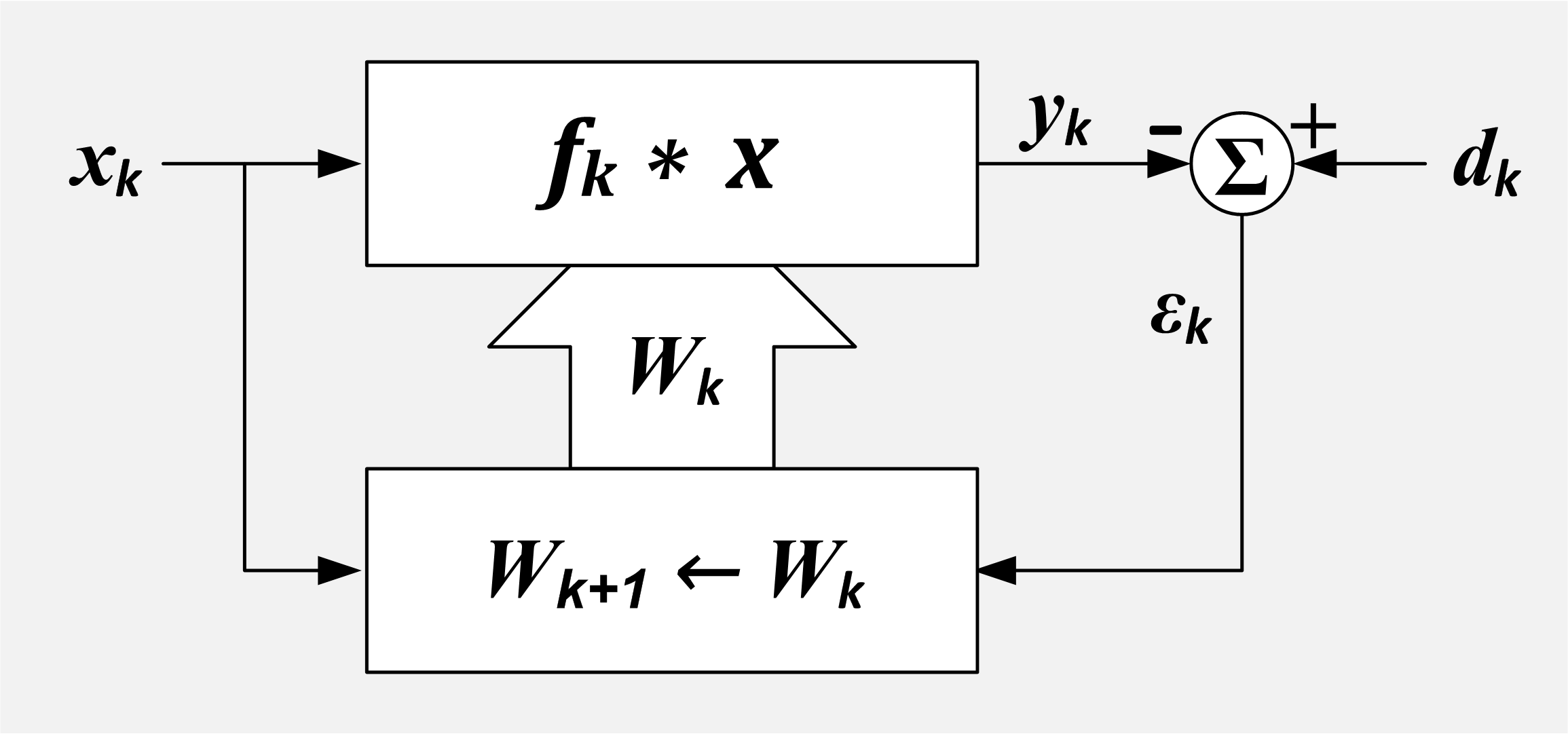
As seen in the diagram, an adaptive filter takes input \(x[k]\), a desired signal \(d[k]#$, and derives filter weights,\)W[k]\(such that the error between the output of the filter,\)y[k]\(and the desired output\)d[k]$$ is minimum. In order to use the adaptive filter in our system, we need to detect the preamble, perform the adaptation process during the duration of the preamble to determine the optimal weights, and then filter the remaining portion of the burst with the derived weights. The input signal is our burst, and the desired signal is the preamble (assumed to be known a-priori when the transmitter and receiver decide on a communications protocol to use). Therefore, the adaptation process derives FIR filter weights such that if the received filter were filtered with the derived filter weights, the reconstructed preamble would be as close as possible to the original preamble in the MMSE sense. As noted above, adaptation stops after the preamble, so a key assumption of this design is that the burst length (in time) is shorter than the coherence time of the channel.
The adaptive filter also has the effect of taking care of synchronization. Intuitively, this makes sense because the FIR filter is adapting to the received signal, which is corrupted due to all effects including sample clock mismatch (which contributes to time synchronization), LO mismatch (which contributes to frequency synchronization), as well as channel effects such as multipath, with the reference signal (desired signal in adaptive filtering parlance) being the properly synchronized and non-noisy preamble.
SDR Implementation
From an implementation perspective, an important point that was glossed over previously is when the adaptive filter begins the adaptive process. It is imperitave that the adaptive filter begin adaptation at the exact sample that the preamble begins in the received signal. If adaptation did not start at the exact sample of the received preamble, the adaptive filter would not generate the correct weights because it is not aligned to the preamble. The reason this must be pointed out when considering implementation becomes clear when we examine the typical signal processing chain for a burst receiver in SDR.
High Level Approach
The first step in a burst processing system is typically a burst detector, which outputs some samples before the burst begins, and some samples after the burst ends. The goal of the burst detector is to prevent the rest of the signal processing chain from processing data that doesn’t contain any information. The input to and output of a burst detector is shown in the figure below, where it can be seen that the input has a lot of extraneous zero’s before and after the burst that are trimmed off by the burst detector.
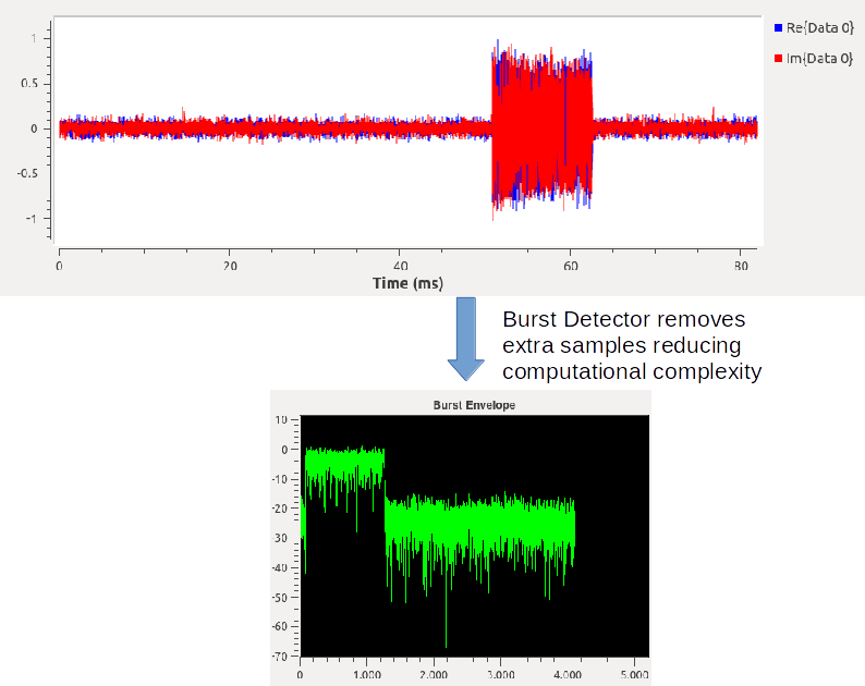
As stated above, is imperative for the adaptive filter to know exactly at which sample it should begin adaptation. After burst detection, it then makes sense to determine the exact start of the preamble. One way to determine this is to perform a cross-correlation of the received signal with the preamble. The peak of the cross-correlation will yield the exact beginning of the preamble. However, the depending on the correlation properties of the preamble, the cross-correlation may not work properly if the signal’s center frequency offset (CFO) is not within some tolerance. Therefore, a safe first step is to perform coarse CFO correction before the cross-correlation. After coarse CFO correction, the exact start of the preamble must be detected, typically with a cross-correlation operation. Finally, after precise detection of the start of the preamble, filtering can be performed to equalize the signal. The processing chain that we now have to perform can be summarized in the following diagram.

Let us now explore how to build each one of these blocks.
Burst Detection
Burst detection is typically implemented as a simple energy threshold mechanism, where the input signal’s energy is calculated. When it rises above a certain threshold that can be determined statically or dynamically, samples are captured and tagged as a burst. Some Matlab code which implements a burst detector is shown below.
inputSigPower = (abs(x).^2)/2; % perform moving average of the signal
kernel = ones(1,maSize)/maSize;
inputSigPowerSmoothed = conv(inputSigPower, kernel);
inputSigPowerSmoothed = inputSigPowerSmoothed(1:length(inputSigPower));
thresh = 3; state = 0; bursts = {}; burstsIdx = 1;

for ii=1:length(inputSigPowerSmoothed)
    if(state==0)
        if(inputSigPowerSmoothed(ii)>thresh)
            burstStartIdx = ii;
            state = 1;
        end
        else if(inputSigPowerSmoothed(ii)<thresh)
            burstEndIdx = ii;
            state = 0;
            % record burst into a vector
            bursts{burstsIdx} = inputSigPowerSmoothed(burstStartIdx:burstEndIdx);
            burstsIdx = burstsIdx + 1;
        end
    end
end
Coarse CFO Estimation and Correction
The next step is to perform coarse CFO estimation and correction. It is known that the information content of an M-PSK signal can be removed by raising the signal to the Mth power. Consequently, because this is a QPSK signal, we can remove the information content of the signal by taking the 4th power of the signal. Taking the FFT of the 4th power of the signal reveals the coarse CFO offset. After detection, the effect of the CFO can be removed by multiplying the signal by a complex exponential.
x4 = x.^4; % take qpsk ^ 4th to extract baudrate lines
X4 = fftshift(abs(fft(x4)).^2);
f = linspace(-Fs/2,Fs/2,length(x4));
[maxVal, maxIdx] = max(X4);
cfoEstimate = f(maxIdx)/4;

to = (0:length(x)-1)/Fs;
freqCorrVector = exp(-j*2*pi*cfoEstimate*to);
y = x.*freqCorrVector;
Determining exact start of Preamble in the received sequence
As discussed above, the next step is to perform a cross-correlation to determine the exact start sample of the preamble. The code sample below shows how to determine the exact start of the preamble using a cross-correlation.
preCrossCorr_cmplx = xcorr(preSyms',eqBurst'); % preSyms is the known preamble symbols, eqBurst is the received symbols
preCrossCorr = abs(preCrossCorr_cmplx);
[maxVal,maxIdx] = max(preCrossCorr);
preambleIdxStart = length(eqBurst) - maxIdx + 1;

eqIn = eqBurst(preambleIdxStart:end); % extract symbols which will be used for equalization (received preamble symbols only)
After performing all of the pre-processing steps, the final step is to perform the adaptive filtering. The adaptive filtering consists of decimating the input signal to rate match what the equalizer is expecting. After rate matching, the optimal filter must be determined. Finally, the optimal filter must be applied and then a simple first order PLL to “clean-up” the output constellation. Let us discuss in detail each of these operations.
Rate Matching
The first step in the adaptive filtering process is to rate-match the data being equalized and the equalizer. By rate-matching, we mean that the equalizer should be designed so that it knows how many samples per symbol it is expecting for its input. Typically, sampling rates of receivers are set to a minimum of 2 samples per second. The choice is whether to design the equalizer such that it accepts the number of samples per symbol that the input signal is sampled at, or to decimate/interpolate the signal to operate at the required number of samples per symbol required by the equalization algorithm. In our specific implementation, we assume that the receiver samples the signal at 2 samples per second, and the equalizer is designed for operating at 1 sample per second. Therefore, we decimate the input signal to accomplish the rate matching.
eqIn_div2 = eqIn(1:2:end); % decimate
Determining the Optimal Filter
In order to determine the optimal filter, we essentially run the adaptive filter shown above. It should be cautioned however that if the training sequence is short, the adaptive filter may not converge to the optimal solution in the amount of available training samples (this is due to many factors, including the learning rate, the amount of noise in the signal, etc..). In order to overcome this, we can apply the closed form solution to the adaptive filter, which ends up reducing to determining the optimal Wiener filter [2]. To determine the optimal Wiener filter, we first create an autocorrelation matrix of the input [3]. This is done by computing the autocorrelation of the input sequence, and then creating a Toeplitz matrix from the autocorrelation sequence. The code below shows how to create the autocorrelation matrix.
[~, d_n] = genPreamble(); % generate the preamble sequence
x_n = eqInput(1:length(d_n));
x_n = x_n(:); % generate the input correlation matrix

X = fft(x_n,2^nextpow2(2*size(x_n,1)-1));
X_magSq = abs(X).^2;
rxx_ifft = ifft(X_magSq);
m = length(x_n);
rxx = rxx_ifft./m; % Biased autocorrelation estimate % creates: http://en.wikipedia.org/wiki/Autocorrelation_matrix

toeplitzMatCol = rxx(1:m);
toeplitzMatRow = conj(rxx(1:m));
R = toeplitz(toeplitzMatCol,toeplitzMatRow);
After creating the autocorrelation matrix, we then create what we call the \(P\) vector. The \(P\) vector is the cross-correlation of the input preamble sequence with the reference preamble sequence. Intuitively, it is a representation of how close the received preamble sequence is to the reference preamble sequence. With the \(P\) vector and the \(R\) matrix, we can setup the filter weight problem as a linear algebra problem. We have \(Pw=R\), and we have to solve for \(w\) which is the optimal weight vector. The code below shows how to accomplish these steps.
xc = xcorr(d_n, x_n);
P_row = xc(1:m);
P = P_row(:); % solve the optimal weights problem w = R\P;
Finally, we scale the weight vector such that the energy of the output of the of the optimal filter is equivalent to the energy of the input vector by scaling such that the maximum input vector tap is 1. The code below shows the filter scaling operation:
wOpt = w./max(abs(w));
Filtering
After determining the filter coefficients, the next step is to filter the actual signal. Filtering can be performed either with an FFT based filter, or a convolution filter. An FFT based filter implementation is shown in the code below:
fftSize = length(eqIn_div2)+length(wOpt)-1;
eqIn_div2_ext = [eqIn_div2 zeros(1,fftSize-length(eqIn_div2))];
wOpt_ext = [wOpt zeros(1,fftSize-length(wOpt))];

whFilt_unscaled = ifft(fft(eqIn_div2_ext).*fft(wOpt_ext));
whFilt_mean = mean(abs(whFilt_unscaled));
whFilt = whFilt_unscaled./whFilt_mean;
PLL (Clean up)
Finally, in order to clean up any residual phase offsets, a simple first order PLL is implemented. The code for the PLL is shown below:
function [ y ] = qpskFirstOrderPLL( x, alpha )
    phiHat = 0;
    y = zeros(1,length(x));

    for ii=1:length(x)
        y(ii) = x(ii)*exp(-j*phiHat); % demodulating circuit
        if(real(y(ii))>=0 && imag(y(ii))>=0)
            % 1 + 1j;
            xHat = exp(1j*pi/2);
        elseif(real(y(ii))>=0 && imag(y(ii))<0)
            % 1 - 1j;
            xHat = exp(1j*3*pi/2);
        elseif(real(y(ii))<0 && imag(y(ii))<0)
            % -1 - 1j;
            xHat = exp(1j*5*pi/2);
        else
            % -1 + 1j;
            xHat = exp(1j*7*pi/2);
        end phiHatT = angle(conj(xHat)*y(ii));
        phiHat = phiHatT*alpha + phiHat;
    end
end
Conclusion
In this post, we have discussed how to implement an equalizer for a bursty QPSK signal. Matlab code samples were shown, showcasing a possible implementation of the burst synchronizer. The working complete Matlab and C++ implementation of this synchronizer (in the GNURadio framework) is located here: https://github.com/gr-vt/gr-burst/. More specifically, the Matlab files to look at for the synchronizer are:
https://github.com/gr-vt/gr-burst/blob/master/matlab/qpskSyncBurst.m https://github.com/gr-vt/gr-burst/blob/master/matlab/qpskBurstCFOCorrect.m https://github.com/gr-vt/gr-burst/blob/master/matlab/weiner_filter_equalize.m https://github.com/gr-vt/gr-burst/blob/master/matlab/qpskFirstOrderPLL.m
For a complete C++ implementation, please see:
https://github.com/gr-vt/gr-burst/blob/master/include/burst/synchronizer_v4.h https://github.com/gr-vt/gr-burst/blob/master/lib/synchronizer_v4_impl.h https://github.com/gr-vt/gr-burst/blob/master/lib/synchronizer_v4_impl.cc
For an example of how to integrate this block into a full-fledged communication system, please see http://oshearesearch.com/2015/04/02/burstpskmodem/
Here is a talk I gave on this at Cyberspectrum meeting in Arlington: [youtube=http://www.youtube.com/watch?v=r64-EA0IneU&t=68m15s]
References
- https://commons.wikimedia.org/wiki/File:QPSK_Freq_Error.svg
- https://en.wikipedia.org/wiki/Wiener_filter
- https://en.wikipedia.org/wiki/Autocorrelation_matrix