PCA, Statistical Whitening, and ICA
Introduction
In this post, I’d like to solidify the concepts of PCA and Statistical Whitening, as well as explain how they relate to ICA. While studying ICA and being a newcomer to the topic, I found that I was confused by how these three important techniques are related to each other. I hope that this post clarifies that to others who may have similar questions. We’ll start by reviewing linear algebra bases, and then discussing PCA, and the intuition behind this algorithm. Next, we will discuss statistical whitening and how it is related to PCA. Finally, we’ll look at ICA and how it relates to both.
Bases (Linear Algebra)
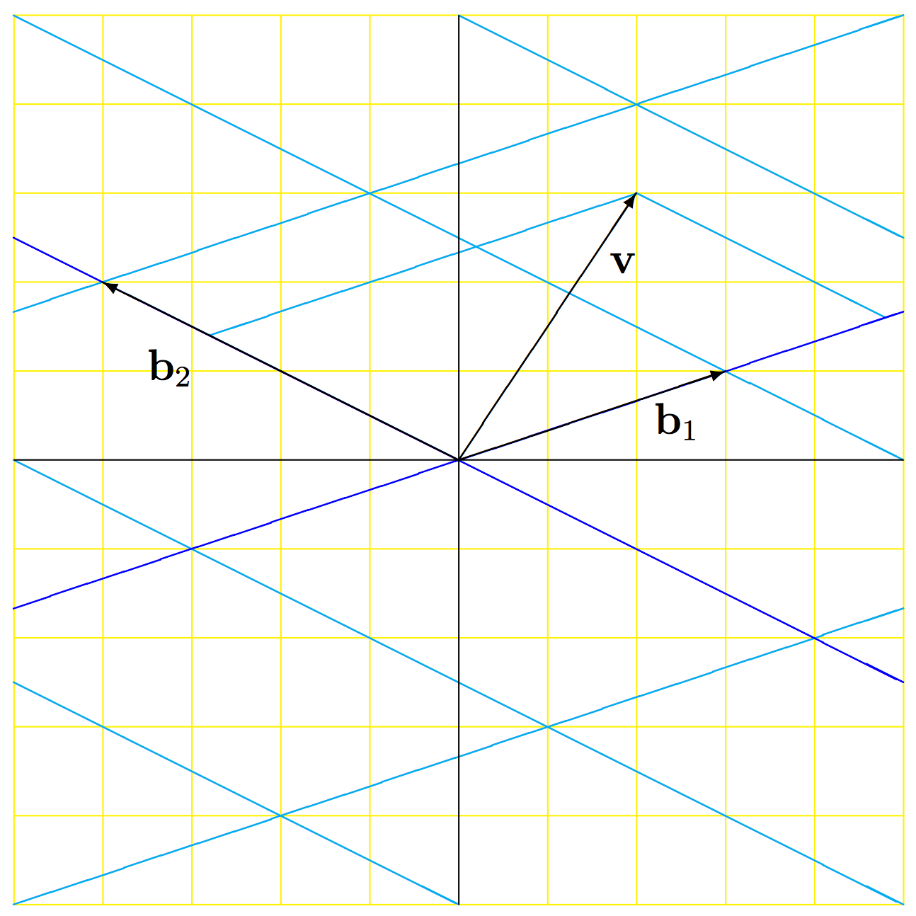
Before we dive into PCA, Whitening, and ICA, it is helpful to review some basic linear algebra concepts about bases. A basis (plural bases), in terms of linear algebra, is a set of linearly independent vectors that can represent any vector in a vector space. One basis for data in \(R^2\) (2 dimensions) is \(\begin{bmatrix} 1 & 0 \\ 0 & 1 \end{bmatrix}\). This basis is also called the standard basis. You can visualize the basis as the axis in the coordinate system on which the data exists. We use bases to represent data in the dimension that the basis covers, and the same data point can be represented by multiple bases. For example, suppose we have data in \(R^2\) and we have two bases to represent the data in, the standard basis \(\begin{bmatrix} 1 & 0 \\ 0 & 1 \end{bmatrix}\) and another basis \(\begin{bmatrix} 3 & {-4} \\ 1 & 2 \end{bmatrix}\). Now, suppose that we have a vector \(\mathbf{v}\), as shown in the figure below. In the figure, the standard coordinates are shown with black axes and a yellow grid, while the \(\beta\)-coordinates are shown with blue axes and a cyan grid. It is easy to see that in the standard basis, we can represent \(\mathbf{v}\) by \((2,3)\). That same vector can also be represented in the \(\beta\) basis as \((1.6,0.7)\) by applying the transformation matrix from the standard basis coordinates. For further details on basis transformation, please refer to this excellent tutorial.

PCA
PCA, which stands for Principal Component Analysis, is a statistical procedure, which at a very high level, can be viewed as an algorithm for finding a more “meaningful” basis for the data to be analyzed. For PCA, meaningful is measured in terms of variance and covariance. A basis vector with higher variance is considered more meaningful than a basis vector with lower variance. The reason this is important is because when we collect multi-dimensional real world data, it is typically corrupted by noise. Additionally, several dimensions (features) of the multi-dimensional data may be redundant. PCA is an algorithm that people use to try to filter out the noise as well as reduce the redundancy in the data set.
Now that we understand what PCA is supposed to do, let’s examine why variance is a part of the measure of meaningfulness of the data. Variance is defined as the spread of a set of numbers from the expected value. A higher variance corresponds directly to more spread, which can be interpreted from an information theoretic standpoint as more informative because inherently the data is harder to predict if it is more spread out (has more entropy). Another way to think about variance is the concept of Signal-to-Noise ratio (SNR). SNR is defined as the ratio of signal power to noise power, which turns out to be the ratio of the variance of the signal to the variance of the noise (because variance is a measure of power). The higher the SNR, the less noisy the signal, or in other terms the “cleaner” the signal. If we make an assumption that in general the data we observe has a reasonable SNR (which is a requirement if we wan’t to do anything with the data to begin with), then high SNR corresponds to a high variance due to how it is defined as a ratio of variances.
The other metric that was defined was covariance. Covariance is a measure of linear dependency between two random variables. If the covariance between two variables was high, this means that they are strongly linearly related. Therefore, having a low covariance implies less (linear) redundancy in the data set. As an aside, I emphasize linearity of the dependency metric here because it is extremely important. People often use the words correlation and dependency synonymously, but that is not statistically accurate except in the Gaussian case! We will explore this topic in more detail in another post, but for now let us continue our discussion of PCA.
Now that we have defined what a more meaningful basis is, how would we design an algorithm to find a more meaningful basis? That is, what mathematical operation(s) can we perform on a data set such that we find directions where the variance is high and the covariance between different dimensions of the data is low? Recall that the variance and covariance information of a multidimensional data set is captured by the covariance matrix. The diagonals of a covariance matrix represent the variances of the individual dimensions, and the off diagonal terms represent the covariance between these variables. Intuitively, what we want is a transformation such that the covariance matrix of the transformed data has diagonal terms that are in descending order (to satisfy the requirement of having a descending order of variances) and has off-diagonal terms as close to zero as possible. Essentially, we’d like to have a transform such that the covariance matrix of the transformed data is diagonal. It is important to note here that a diagonal covariance matrix means that the features of the data are no longer correlated. Therefore, another way to state the algorithmic goals of PCA are to find a decorrelation matrix, which in our context rotates the data from a naive basis to a more meaningful one.
So how do we find a decorrelation matrix? Suppose our data is in a matrix \(\mathbf{X} \epsilon \mathbb{R}^{n x d}\), where \(d\) is the number of features, and \(n\) is the number of data points captured for each feature. The covariance matrix of \(\mathbf{X}\) is then calculated as \(\Sigma_{X} = E[XX^T]\). We now desire a transform matrix \(\mathbf{P}\) such that the covariance of \(\mathbf{PX}\) is diagonal. Armed with this intuition (and skipping a few steps), we find that \(\mathbf{P} = \mathbf{E^T}\), where \(\mathbf{E}\) is the matrix of eigenvectors of \(\mathbf{X}\).
Statistical Whitening Transform
The statistical whitening transform is a set of operations performed on a multivariate data set which results in a decorrelated data set that has uniform variances on all diagonals. Recall that PCA also results in a decorrelated data set, but the variances are not uniform. In fact, the variances of a data set transformed by PCA are in descending order (recall that this was a requirement of PCA). Intuitively then, we can achieve statistical whitening by first performing PCA, and then multiplying by another matrix such that the diagonal’s of the resultant data set’s covariance matrix are unity. Even though it wasn’t shown mathematically above, the diagonals of the PCA’ed covariance matrix correspond to the eigenvalues of \(\mathbf{X}\), which are stored in a matrix \(\mathbf{D}\). It can be shown that left multiplying by \(\mathbf{D^{1/2}}\) has this effect. Therefore, statistical whitening of a dataset in matrix \(\mathbf{X}\) can be achieved as follows: \(\mathbf{Y} = \mathbf{D}^{1/2} \mathbf{E}^T \mathbf{X}\), where \(\mathbf{Y}\) is the whitened data.
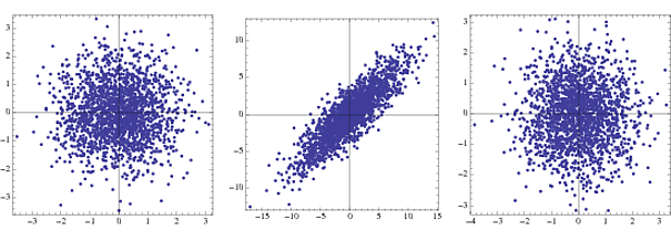
Whitening is also sometimes referred to as sphering, because of the resultant shape of the data. In the figure, the left figure is the joint density of two uncorrelated Gaussian random variables, the middle is the joint density of two correlated Gaussian random variables with differing variances, and the sub-figure on the right shows the output of the whitening transform on the middle data set.

ICA
Now that we understand PCA and its relation to statistical whitening, let us explore ICA and see how these concepts relate to each other. ICA, which stands for Independent Component Analysis, is a statistical procedure which attempts to separate sources which are mixed together through properties of statistical independence. One interpretation of ICA is similar to PCA, in the sense that it tries to extract the most “meaningful” basis for representing the multivariate data set. However, instead of using variance and covariance as a means of measuring the meaningfulness of a basis as was done in PCA, it uses statistical independence.
We won’t delve into the details of ICA here, but rather the goal is to explain how PCA and Statistical Whitening fit into the ICA algorithm. However, we do need to discuss some of the math behind ICA. Mathematically, ICA can be expressed in the equation \(\mathbf{x} = \mathbf{As}\), where \(\mathbf{x}\) is the observed vector of data, and we try to recover \(\mathbf{s}\) without knowledge of \(\mathbf{A}\). For this to be a tractable problem, several assumptions need to be made. One is that the sources, represented by \(\mathbf{s}\) are statistically independent. Another important assumption is that the sources are Non-Gaussian (although that will not be germane to our discussion here). Finally, the sources are all assumed to be of unit variance. In practice, although data may not be present in nature with unit variance, it can always be transformed to achieve unit variance, so this isn’t really an “assumption.” With this background, let us proceed mathematically.
Because the sources were assumed to be independent and unit variance, we know that the covariance matrix of the sources should be the identity matrix, i.e. \(E[\mathbf{s}\mathbf{s^T}] = \mathbf{I}\). Now, computing the covariance matrix of the observed data matrix, some substitutions can be made as follows: \(E[\mathbf{x}\mathbf{x^T}] =E[\mathbf{As}\mathbf{\left(As\right)^T}] =E[\mathbf{As}\mathbf{s^TA^T}] = E[\mathbf{A}\mathbf{A^T}] =\mathbf{AA^T}\). Recall from linear algebra that any matrix can be decomposed using Singular Value Decomposition (SVD). Let us suppose that \(\mathbf{A} = \mathbf{U}\Sigma \mathbf{V^T}\), which is the SVD of \(\mathbf{A}\). Substituting into our previous expression and simplifying, we get that \(E[\mathbf{x}\mathbf{x^T}] = \mathbf{U}\Sigma^2 \mathbf{U^T}\). We also know that \(E[\mathbf{x}\mathbf{x^T}] = \mathbf{EDE^T}\) (through eigenvalue decomposition). Therefore, we can set the following relation: \(\mathbf{EDE^T} =\mathbf{U}\Sigma^2 \mathbf{U^T}\). This implies that \(\mathbf{E} = \mathbf{U}\) and \(D = \Sigma^2\), which implies that \(\Sigma^{-1} = \mathbf{D}^{-1/2}\).
At this point, it is good to take a step back and realize that in essence, what we are trying to solve for is the unknown mixing matrix \(\mathbf{A}\). If we knew \(\mathbf{A}\), then we could compute its inverse and plug into our original equation to recover \(\mathbf{s}\). From the SVD decomposition of \(\mathbf{A}\), we can write that \(\mathbf{A}^{-1} = \mathbf{V}\Sigma^{-1} \mathbf{U^T}\). Substituting the relations we found above, we can show that \(\mathbf{A}^{-1} = \mathbf{VD^{-1/2}} \mathbf{E^T}\). From our discussion of PCA and statistical whitening, we know that \(\mathbf{E}^T\) is the decorrelation matrix (i.e. the PCA algorithm), and that \(\mathbf{D}^{-1/2}\) is the whitening matrix. Since these are the first two operations applied to the observed vector \(\mathbf{x}\), we can interpret the first two steps of ICA as performing PCA and then statistical whitening. The final step is the estimate \(\mathbf{V}\) such that the output sources are statistically independent.
Conclusion
In this blog post, we have shown how PCA, Statistical Whitening, and ICA are related to each other. I hope this has been helpful and clarifying to others studying this field.
References
- https://arxiv.org/pdf/1404.1100.pdf (More in depth tutorials of PCA)
- https://www.cs.helsinki.fi/u/ahyvarin/papers/NN00new.pdf (Very in depth tutorial on ICA)